Training Strategy

This section describes the training configuration, data preparation pipeline, and optimization strategies for RTnn.

Data Preparation

RTnn processes NetCDF files containing LSM data with the naming convention: rtnetcdf_{processor_rank:03d}_{year}.nc

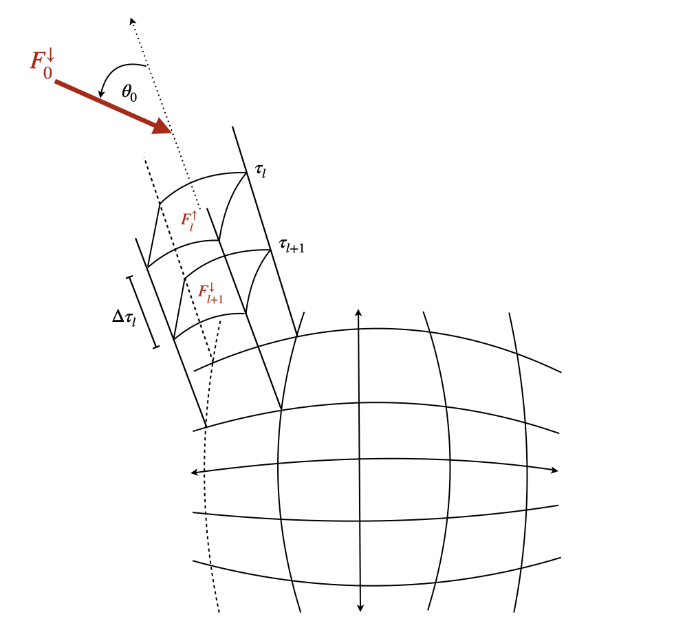
Structure of the vegetation canopy

Vertical Canopy Structure:

The model simulates radiative transfer through multiple vertical layers (default: 10 layers), representing different heights within the vegetation canopy. Each layer has its own optical properties (leaf area index, single scattering albedo, etc.) that influence radiation propagation.

Processor Rank Distribution:

Data is distributed across multiple processor ranks (for example 16 ranks). For training, a random subset (60%) is selected in each epoch to reduce bias and improve generalization.

Example of randomly selected MPI blocks used during training

Random Spatial Mapping:

• During training, a new random spatial mapping is generated for each time step

• 60% of processor ranks are randomly selected (data augmentation)

• The same mapping applies to all spatial batches within a time step

• Validation/testing uses 100% of processor ranks (deterministic)

Input Features (121 channels):

The input features are constructed from four variable groups, flattened across Plant Functional Types (PFTs, 15 types) and spectral bands (2 bands: VIS and NIR):

Input Channel Composition

Variable Group	Channels	Description
coszang	1	Cosine of solar zenith angle (direct beam direction)
laieff_collim, laieff_isotrop	30 (2 × 15 PFTs)	Leaf area index for collimated and isotropic radiation
leaf_ssa, leaf_psd	60 (2 × 2 bands × 15 PFTs)	Single scattering albedo and phase function asymmetry
rs_surface_emu	30 (1 × 2 bands × 15 PFTs)	Surface reflectance (soil albedo)
Total	121

Output Targets (120 channels):

The model predicts four output variables for each PFT and band combination:

Output Channel Composition

Variable Group	Channels	Description
collim_alb	30 (15 PFTs × 2 bands)	Collimated albedo (reflected direct radiation)
collim_tran	30 (15 PFTs × 2 bands)	Collimated transmittance (transmitted direct radiation)
isotrop_alb	30 (15 PFTs × 2 bands)	Isotropic albedo (reflected diffuse radiation)
isotrop_tran	30 (15 PFTs × 2 bands)	Isotropic transmittance (transmitted diffuse radiation)
Total	120

Physical Constraint:

For each layer, the outputs satisfy energy conservation:

\[\text{albedo} + \text{transmittance} + \text{absorption} = 1\]

This constraint is enforced as a soft penalty during training.

Hyperparameters

Learning Rate

--learning_rate 0.0001

Recommendations:

• LSTM/GRU: 1e-3 to 1e-4

• Transformer: 1e-4 to 5e-5

• VerticalRT: 1e-4 to 5e-5

Batch Size

--batch_size 4
--tbatch 24  # 24 temporal batch size for the validation, and 1 for inference

Note: For VerticalRT with 120 output channels, reduce batch size to 4-8 due to memory constraints.

Loss Functions

--loss_type huber
--beta 0.2  # Weight for absorption loss
--beta_delta 1.0  # For Huber/SmoothL1

Loss Function Options:

Loss Function Types

Loss Type	Best For	Description
mse	General purpose	Standard Mean Squared Error
mae	Robust to outliers	Mean Absolute Error
huber	Balanced	Combines MSE and MAE
smoothl1	Similar to Huber	Smooth L1 Loss
nmae	Scale-invariant	Normalized MAE
nmse	Scale-invariant	Normalized MSE

Weighted Loss Formula:

\[\mathcal{L}_{\text{total}} = (1 - \beta) \cdot \mathcal{L}_{\text{fluxes}} + \beta \cdot (\mathcal{L}_{\text{abs12}} + \mathcal{L}_{\text{abs34}})\]

Where: - \(\beta\) controls the trade-off between flux accuracy and absorption accuracy - Typical \(\beta\) values: 0.05 - 0.3

Learning Rate Scheduling

RTnn uses ReduceLROnPlateau scheduler:

scheduler = ReduceLROnPlateau(
    optimizer,
    factor=0.5,      # Reduce LR by 50%
    patience=5,      # Wait 5 epochs before reducing
    mode='min'       # Monitor validation loss minimum
)

The learning rate is reduced when validation loss plateaus.

Optimizer

Adam optimizer with default parameters:

optimizer = torch.optim.Adam(
    model.parameters(),
    lr=learning_rate
)

Training Tips

For LSTM/GRU:

• Hidden size: 128-256 for 121 inputs

• Number of layers: 2-4

• Dropout: 0.2-0.4

For Transformer:

• Embed size: 256-512

• Number of heads: embed_size // 64

• Forward expansion: 2-4

• Dropout: 0.1-0.3

For VerticalRT:

• Hidden size: 256

• Layer embedding dimension: 16

• Dropout: 0.1

General Tips:

1. Start with smaller learning rate (1e-4) for larger models

2. Use gradient clipping for stable training

3. Monitor conservation penalty (should approach 0)

4. Save checkpoints every 10 epochs

5. Use mixed precision training for memory efficiency

See Neural Architectures for architecture-specific details.